Barkane's Stylistic Volumetric Clouds

§ Overview

The endgoal of this walkthrough is to generate cotton-like 3D clouds

↗
The constraints are
- Viewing angle: because the player can freely rotate around the world, clouds could be viewed at any angle, not just from the bottom
- Occlusion: the cloud must fit well in front of changing skyspheres and in-game objects
This could not be fulfilled completely, see later sections for details
- Cost: as clouds are purely cosmetic, they should not take up too much computation comparing to the rest of the game
- Variation: clouds should be unique enough when several are placed together
- Stylistic: ultimately, the cloud should look like a cartoon cotton ball more than actual clouds
Naturally there are several approaches, and the main decision boils down to choosing between 2D and 3D noise textures. 3D noise is preferred because it provides the most nuance in different viewing angles.
This decision creates several issues, namely
- How to generate 3D noise textures
- How to sample from 3D noise textures
- How to stylize the samples
The rest of the walkthrough will go over the development process and focus on how these issues are solved

Formulas borrow heavily from this presentation by Andrew Schneider from Guerrilla Games

§ Generating 3D Worley Noise

Typically for any generated rendering, nuance (i.e. non-repetitive details) comes from manually added details or random noise
For clouds, the "nuance" is the density distribution of the cloud itself
- In games with open sky scenes, clouds are usually one large sheet. The density applies throughout that sheet and additional techniques are used to "carve" clouds out of the sheet. However for Barkane clouds are individual objects, so the "carving" sections of referenced papers can more or less be skipped.
- The only relevant noises are Perlin and Worley noises, for simplicity's sake
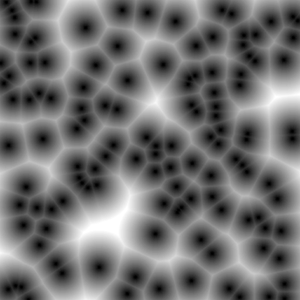
A Worley noise is a noise based on seed points, the value at each point of the sample space is the distance to the closest seed point in that entire space (image from Wikipedia)

↗
- The inverted version with several round "dots" in each "cell" is ideal for rendering cotton

There are various examples online for creating 3D Worley noise directly from a 3D compute shader

This shader by Jushii Tuomi

However, for compatibility and performance concerns this walkthrough uses serialized 2D texture slices and combines them at runtime to form the 3D texture. This removes the need to run compute shaders inside the game.

Also, the noise generated below will not be inverted within the texture. This is to make sure it can be used as normal Worley noise in other contexts.

§ The 2D Compute Shader

The skeleton code of a 2D compute shader is as follows
```
# pragma kernel CSWorley
RWTexture2D<float4> _Result;
[numthreads(8, 8, 1)]
void CSWorley(uint3 id: SV_DispatchThreadID) {
  _Result[id.xy] = float4(id.x, id.y, id.z, 0);
}
```
which just writes the current thread position into the _Result buffer

For more about thread indices, here is a Microsoft doc about it. The main idea is each thread has a 3D coordinate with each dimension going from 0 to resolution

Some extra data must be added to the input

int _Width; // Number of cells along one axis of the texture (all unit length)
int _Density; // How many samples per cell
float _z; // the current slice

// The seed points, StructuredBuffer is used to transfer data from the C# program (in the CPU) to the shader (in the GPU)
StructuredBuffer<float3> _Pts;

// 3D cell offsets, reference from Jushii Tuomi https://github.com/jushii/WorleyNoise/blob/main/Assets/Shaders/Worley3D.compute
static const int3 offsets[] =
{
  int3(-1, -1, -1),
  int3(0, -1, -1),
  int3(1, -1, -1),
  int3(-1, -1, 0),
  int3(0, -1, 0),
  int3(1, -1, 0),
  int3(-1, -1, 1),
  int3(0, -1, 1),
  int3(1, -1, 1),
  int3(-1, 0, -1),
  int3(0, 0, -1),
  int3(1, 0, -1),
  int3(-1, 0, 0),
  int3(0, 0, 0),
  int3(1, 0, 0),
  int3(-1, 0, 1),
  int3(0, 0, 1),
  int3(1, 0, 1),
  int3(-1, 1, -1),
  int3(0, 1, -1),
  int3(1, 1, -1),
  int3(-1, 1, 0),
  int3(0, 1, 0),
  int3(1, 1, 0),
  int3(-1, 1, 1),
  int3(0, 1, 1),
  int3(1, 1, 1),
};

In the CSWorley kernel, we first figure out the cell index of the current thread based on its thread index. (Note that the z coordinate is injected instead of using the thread index)

float fWidth = (float)_Width;
float fDensity = (float)_Density;

float3 raw = float3(id.x, id.y, _z); // XYZ position in [0, _Width * _Density) range
float3 pos = raw / fDensity; // Grid position in [0, _Width) range
int3 cell = floor(pos); // cell index in [0, _Width) range

float sqMin = 100000f; // some very large value that guarantees to be updated later

Then, for each neighboring cell, we compute the distance from the current sampling point to the seed point in that cell

for (int i = 0; i < 27; i++) {
  int3 neighbor = cell + offsets[i]; // the neighbor's cell's position
  int3 samplingCoordinate = neighbor;
  int ptIdx = samplingCoordinate.x + _Width * (samplingCoordinate.y + _Width * samplingCoordinate.z);

  float3 toNeighbor = neighbor - pos; // distance from current sample to the neighboring cell (not the neighboring cell's seed point)
  float3 displacement = _Pts[ptIdx] + toNeighbor; // distance from current sample to the neighboring seed point

  sqMin = min(sqMin, dot(displacement, displacement)); // squared distance

  // ...
}

However, this actually leads to out of bounds errors since
- A negative offset on the 0th cell results in a negative index
- A positive offset on the last cell results goes out of bounds of the _Pts buffer

To fix this, we first introduce some helper functions

bool legal(int dim) {
  return dim >= 0 && dim < _Width;
}

bool legal(int3 dims) {
  return legal(dims.x) && legal(dims.y) && legal(dims.z);
}

int idx(int3 dims) {
  return dims.x + _Width * (dims.y + _Width * (dims.z));
}

Then we apply those helper functions inside the CSWorley loop
```
// ...
int3 neighbor = cell + offsets[i];
int3 samplingCoordinate = neighbor;

if (!legal(neighbor)) samplingCoordinate = (neighbor + fWidth) % fWidth;

// ...
```
- Instead of just ditching the sample, we loop the sample with % so that negative indices sample from the back of the buffer and vice versa
Finally, we write the result back to the _Result buffer so it transfers back to the CPU
```
_Result[id.xy] = float4(sqMin, 0, 0, 0);
```
Note that instead of comparing the euclidian distance we compared the squared distance (result of the dot product). That distance is in the range from 0 to sqrt(3) instead of 0 to 1
- The sqrt(3) comes from the fact that we are using cube cells and the diagonal of that is sqrt(3)
- Instead of doing sqrt(sqMin) / sqrt(3) it is simpler to just use sqrt(sqMin / 3)
```
_Result[id.xy] = float4(sqrt(sqMin / 3), 0, 0, 0);
```

§ Channel Usage

Note that the current shader only uses the R channel of the _Result buffer, while the 3 other channels are just empty

To utilize these other channels, 4 separate sets of seed points could be used to create 4 unique black and white textures

[numthreads(8, 8, 1)]
void CSWorley(uint3 id : SV_DispatchThreadID)
{
  float fWidth = (float)_Width;
  float fDensity = (float)_Density;

  float3 raw = float3(id.x, id.y, _z);
  float3 pos = raw / fDensity;
  int3 cell = floor(pos);

  float4 sqMin4 = float4(10000, 10000, 10000, 10000);
  for (int i = 0; i < 27; i++) {
    int3 neighbor = cell + offsets[i];
    int3 samplingCoordinate = neighbor;

    if (!legal(neighbor)) samplingCoordinate = (neighbor + fWidth) % fWidth;

    int ptIdx = samplingCoordinate.x + _Width * (samplingCoordinate.y + _Width * samplingCoordinate.z);

    float3 toNeighbor = neighbor - pos;

    float3 displacement1 = _Pts1[ptIdx] + toNeighbor;
    float3 displacement2 = _Pts2[ptIdx] + toNeighbor;
    float3 displacement3 = _Pts3[ptIdx] + toNeighbor;
    float3 displacement4 = _Pts4[ptIdx] + toNeighbor;

    sqMin4 = float4(
      min(sqMin4.x, dot(displacement1, displacement1)),
      min(sqMin4.y, dot(displacement2, displacement2)),
      min(sqMin4.z, dot(displacement3, displacement3)),
      min(sqMin4.w, dot(displacement4, displacement4)));
  }
  _Result[id.xy] = sqrt(sqMin4 / 3.0);
}

§ Shader Invocation And Texture Saving

Checkout this Unity document for relevant concepts

Note that the compute shader only uses random points, but it never actually generates them
The actual generation happens in another C# script and gets sent over to the compute shader's buffers

Each set of seed points is generated by

ComputeBuffer PtsBuffer(int width)
{
  var numCells = width * width * width;
  // sizeof(float) is used instead of sizeof(Vector3) because latter is not provided
  var buf = new ComputeBuffer(numCells, sizeof(float) * 3, ComputeBufferType.Structured);
  var pts = new Vector3[numCells];
  for (int i = 0; i < numCells; i++)
      // relative location in the cell, in the range (0, 1)
      pts[i] = new Vector3(Random.value, Random.value, Random.value);
  buf.SetData(pts);
  return buf;
}

And to invoke the shader

void Generate(int width, int density, ComputeShader shader)
{
  var resolution = width * density;

  // the resulting 3D texture
  var t3D = new Texture3D(resolution, resolution, resolution, TextureFormat.RGBA32, false)
  {
    wrapMode = TextureWrapMode.Repeat
  };

  // setting relevant data
  var (pts1, pts2, pts3, pts4) = (PtsBuffer(width), PtsBuffer(width), PtsBuffer(width), PtsBuffer(width));

  shader.SetInt("_Width", width);
  shader.SetInt("_Density", density);
  shader.SetBuffer(0, "_Pts1", pts1);
  shader.SetBuffer(0, "_Pts2", pts2);
  shader.SetBuffer(0, "_Pts3", pts3);
  shader.SetBuffer(0, "_Pts4", pts4);

  // one slice
  var rt2D = new RenderTexture(resolution, resolution, 0)
  {
    enableRandomWrite = true,
    filterMode = FilterMode.Point
  };
  rt2D.Create();

  // serialization method, will elaborate later
  BakeTexture(t3D, rt2D, shader, resolution);

  // saving the 3D texture as an asset
  AssetDatabase.CreateAsset(t3D, $"Assets/Materials/Noise/{ShaderName}.asset");
  AssetDatabase.SaveAssets();

  // destroying allocated resources so Unity doesn't throw allocation errors
  #region release
  DestroyImmediate(rt2D);
  pts1.Release();
  pts2.Release();
  pts3.Release();
  pts4.Release();
  #endregion

}

void BakeTexture(Texture3D t3D, RenderTexture rt2D, ComputeShader shader, int resolution)
{
  // get rendertexture to render layers to this 2D slice
  // then, 2D slices are transferred to a 1D array
  // the 1D array is used to create the 3D texture
  var temp = new Texture2D(resolution, resolution)
  {
    filterMode = FilterMode.Point
  };

  // serializing to a 1D array
  var area = resolution * resolution;
  var volume = area * resolution;
  var colors = new Color[volume];

  shader.SetTexture(0, "_Result", rt2D);

  //loop through slices
  for (var slice = 0; slice < resolution; slice++)
  {
    // get shader result
    // the original implementation uses Blit (Material-based), this is switched to the newer Compute Shader version of Dispatch
    shader.SetFloat("_z", slice);
    // the numbers here needs to match the `numthreads` tag in the compute shader
    shader.Dispatch(0, resolution / 8, resolution / 8, 1);

    // write the render texture into the 2D slice
    RenderTexture.active = rt2D;
    temp.ReadPixels(new Rect(0, 0, Resolution, Resolution), 0, 0);
    temp.Apply();
    RenderTexture.active = null;

    // 1D representation of the current slice
    var sliceColors = temp.GetPixels32();

    // transfer it to the 1D representation of the 3D texture
    var sliceBase = slice * area;
    for (var pixel = 0; pixel < area; pixel++)
    {
      colors[sliceBase + pixel] = sliceColors[pixel];
    }
  }

  // force the 3D texture to update before saving it in Generate
  t3D.SetPixels(colors);
  t3D.Apply();

  // similarly, temporary allocated resources are destroyed
  DestroyImmediate(temp);
}

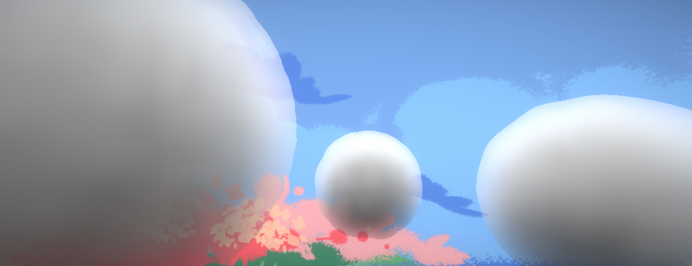
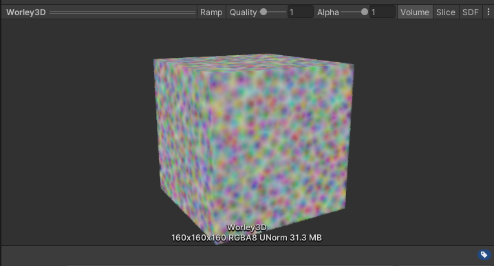
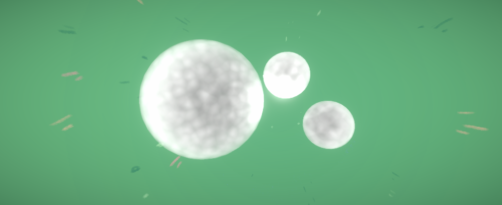
The result using _Width=16 and _Density=10 is as follows

↗

§ Ray-Marching

The original code is based on Unity and more specifically the Universal Render Pipeline. The following technical details are omitted, but feel free to look up the Unity forums for relevant information to

Incorporate shader code into URP + Shader Graph

Get light position from within the shader / Passing light position to the shader

The code in Barkane had to deal with duplicate parameters. For example, function A needs a1, a2 but it also calls B that needs b1, b2, so it ends up being in the form void A(a1, a2, b1, b2) and void B(b1, b2) which is really redundant. For brevity I am going to write functions like these in the form void A(a1, a2) void B(b1, b2).

This section will go over the ray march method itself, the rest of the cloud shader will be explained in the sections below
- This section references:
  - Shaders from this project by Sebastian Lague
  - Code from the appendix of this paper by Fredrik Häggström, starting from B.6
  - Formulas from this presentation by Andrew Schneider from Guerrilla Games

§ Theory

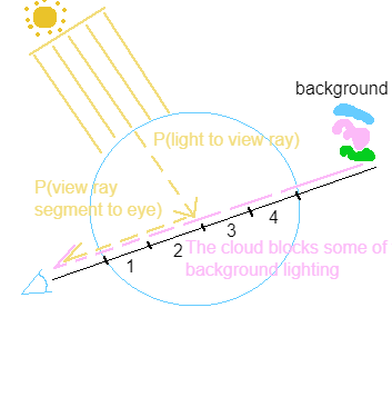
Before any stylization, rendering a cloud is equivalent with computing the amount of light travelling from a point on the cloud to a pixel on the screen

↗
- P(something) denote the probability of something happening
This is an approximation of scattering, or light bouncing between particles within the cloud
- In a general sense, light is less likely to travel along a ray the deeper the ray goes into the cloud, since part of it gets bounced into other directions
- The more particles there are along the ray, there are more objects to bounce the light ray away
  - To count the number of particles, ray-marching is needed to sample the density of the cloud at different points. linear density * length = mass.
  - Whenever we need to find this probability also called transmittance, we will need to add ray-marching to the shader.
- Later sections will go into depth for computing this probability
In this simplified model, light travels...
- From the sun to the view ray, and then "bounced" at the intersection to a direction following the view ray
  - This is then approximated by only sampling a few points at the end of each view ray, rather than all points on the view ray
- From the background to the camera, partially blocked by the cloud

§ Relevant Values

v, the normalized view direction that goes from the eye to the point on the cloud (in object space)
p, the position vector that goes from the center of the cloud (object space (0, 0, 0)) to the point on the cloud (in object space)
l, the light-facing direction that goes from the point on the cloud to the sun (in object space)
- The sun is visualized as an infinite plane, so this is just taking the opposite of where the sun "points" towards
r, the object space length of the radius, set to 0.5 to accommodate Unity's default sphere model

Any other values introduced are parameters of the shader. You can either pass them in as parameters or insert magic numbers in the code (which is not recommended). For brevity they will be used in the code but not written as parameters.

§ Marching

The two marching functions are just logical translations of what's stated in the theory section

Along the view ray

// returned values:
// - cloudColor: RGB colors of the cloud
// - transmittance: overall transmittance of the cloud
void march(float3 p, float3 v, float3 l, out float3 cloudColor, out float transmittance) {
  // The view ray enters the cloud at p, we need to find where it exits
  // The spherical shape allows a quick solution using quadratic formula (derivation omitted)
  float I = dot(v, p);
  float end = -I;
  I = I * I - dot(p, p) + r * r;
  if (I < 0) discard; // the ray does not actually enter the cloud
  end += sqrt(I);

  float energy = 0; // start with no light, gradually accumulate this value
  transmittance = 1; // start with totally transparent, gradually decrease this value

  const float stepSize = end / steps;
  for(uint i = 0; i < steps; i++) {
    const float t = stepSize * (i + 1);
    const float3 pSample = p + t * v; // the current position of the view ray in the cloud
    const float density = densityAt(p); // will elaborate in later sections
    const float mass = density * stepSize * cloudAbsorption; // cloudAbsorption is a stylistic constant
    const float sunTransmittance = sunMarch(pSample, l); // transmittance from sun to view ray, will elaborate below
    
    energy += mass * transmittance * sunTransmittance; // light accumulated on this segment of the view ray
    transmittance *= beer(mass * cloudAbsorption); // this segment blocks light coming from later steps, will elaborate in later sections
  }

  const float4 backgroundColor = panoramic(v); // sampling the skysphere for background lighting, explanation omitted 

  cloudColor = backgroundColor.xyz * transmittance + energy * sunColor;
}

From the light to the view ray

float sunMarch(float3 p, float3 l) {
  // similar endpoint calculation
  float I = dot(l, p);
  float end = -I;
  I = I * I - dot(p, p) + r * r;
  if (I < 0) return 1; // completely transparent if the ray doesn't enter the cloud, this shouldn't really happen
  end += sqrt(I);
  
  const float stepSize = end / steps;
  float mass = 0;
  for(uint i = 0; i < steps; i++) {
    float t = stepSize * (i + 1);
    float3 pSample = p + l * t;
    mass += stepSize * densityAt(pSample);
  }

  return beer(mass * sunAbsorption); // sunAbsorption is a stylistic constant
}

Note that step sizes are calculated in object space, this isn't actually physical (since scale needs to be taken account of in stepSize) but ensures uniformity between clouds of different sizes. Smaller clouds will not appear see-through even though they should in a more physical render.
Here beer refers to Beer's Law: T = e^(-m) (i.e. light is bounced away by cloud mass so transmittance T decreases)

Schneider's presentation explored something they call "beer-powder approximation" which did not really fit the style of Barkane and was skipped. Beer's Law is just a starting point!
The cloudAbsorption value decides the overall brightness, and the sunAbsorption decides the top-bottom brightness difference
- Low sunAbsorption
  
  ↗
- High sunAbsorption
  
  ↗
As a side note, the material itself is set to unlit transparent with the alpha value set to 1 - transmittance

§ Scattering

So far, the cloud's looks are entirely dependent on the density

↗
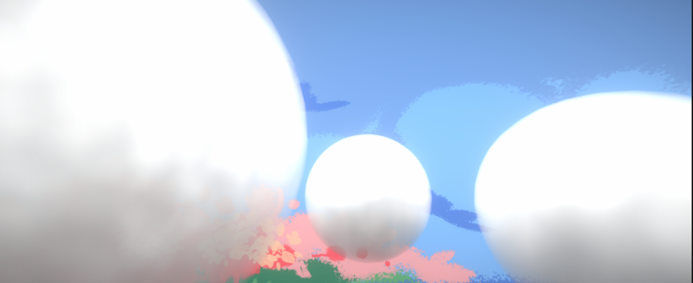
While the leveled view might be fine, views from extreme angles look really dull

↗
- There is no silver-lining that is characteristic of clouds
To correct this, Mie scattering needs to be added into the light accumulation process
- When added, lining up v and l will create strong highlights. This is similar to looking at the sun through the cloud.
- Mie scattering is approximated by the Henyey-Greenstein phase function that takes in an angle (between the view direction and the light direction) and outputs a modifier to the light intensity
```
float hg(float cosa, float g) {
  float g2 = g * g;
  return (1 - g2) / (4 * 3.1415 * pow(1 + g2 - 2 * g * cosa, 1.5));
}
```
- And inside the marching method...
```
const float cosa = dot(v, l);
const float phaseVal = hg(cosa, g);
energy += stepSize * density * transmittance * lightTransmittance * phaseVal;
```
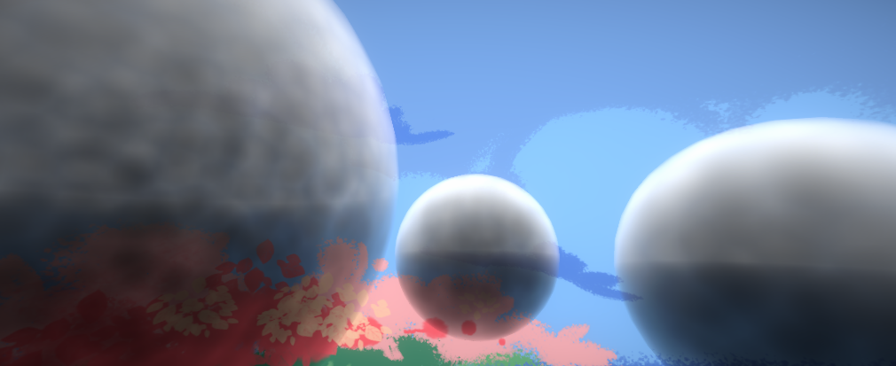
This gives the clouds silver lining when looking from below, but what about above?
- The solution is to add a negative HG term that gives highlight when viewed along the sun's direction
- The two terms are combined by averaging
```
float twoTermHG(float t, float g1, float g2, float cosa, float gBias) {
  return lerp(hg(cosa, g1), hg(cosa, -g2), t) + gBias;
}
```
- And inside the marching method...
```
const float phaseVal = twoTermHG(0.5, g1, g2, cosa, gBias);
```
  Where g1 stands for the forward scattering constant, g2 stands for the backward scattering constant.
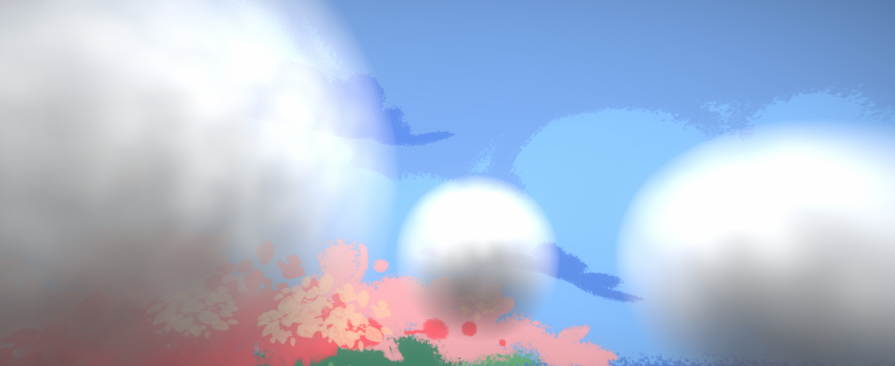
Forward scattering preview
↗
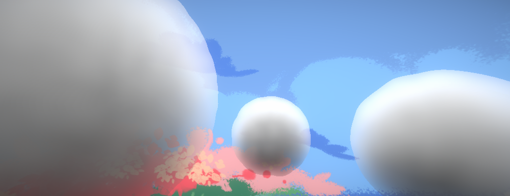
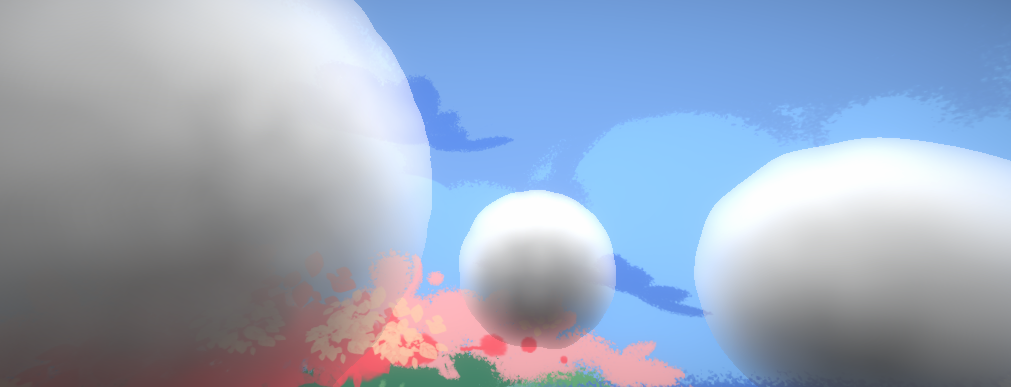
Backward scattering preview (the highlight between the first two clouds from the left)
↗
Generally, larger values of g give smaller and more energized highlights

Another type of scattering that affects the color of the light is called Rayleigh scattering. This is skipped in Barkane because of stylistic reasons.

§ Density

In previous previews, densityAt is substituted with sampling the 3D texture directly

It is better to add a dropoff function that smoothly transitions out of the cloud

float densityDrop(float3 p, float dropoff) {
  float sq = dot(p, p);
  float t = sq / r;
  return exp(-dropoff * t) - exp(-dropoff); // the subtraction makes sure it is zeroed at 1
}

Where dropoff is some value greater than 1. The larger the value the more dramatically density drops.

The entire densityAt
```
float densityAt(float3 p) {
  float3 pWorld = mul(unity_ObjectToWorld, float4(p, 1)).xyz;
  pWorld = pWorld * scl;

  return baseDensity
    * (weights.x + weights.y
      // originally the negation is built into the worley generation shader
      // it is moved here to make the worley noise texture itself more usable elsewhere
      - weights.x * worley.Sample(worleyState, pWorld).r
      - weights.y * worley.Sample(worleyState, pWorld).g);
    * densityDrop(p, densityDropoff);
}
```
- Here the ObjectToWorld transform is needed to make the noise resolution uniform between differently scaled clouds
- scl is the scale of the noise
- worley.Sample(worleyState, pWorld) samples the 3D noise with a sampler state and a position. This is what I found that works with Shader Graph, where the following parameters are passed from the graph itself
  - UnitySamplerState worleyState
  - UnityTexture3D worley
- I found the 2 channel (R and G) enough. If you want more detailed noise feel free to add the B and W channels as well
  - The 2 channels are sampled separately. You can also write this frequency difference into the texture itself and sample both channels in one call. This requires a slightly more complicated compute shader invocation.
↗

§ Stylization

This section goes over additional steps specifically for stylizing. Previous steps are also stylized, just not specifically written for it.

§ Cutoff

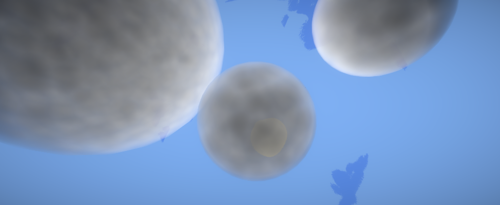
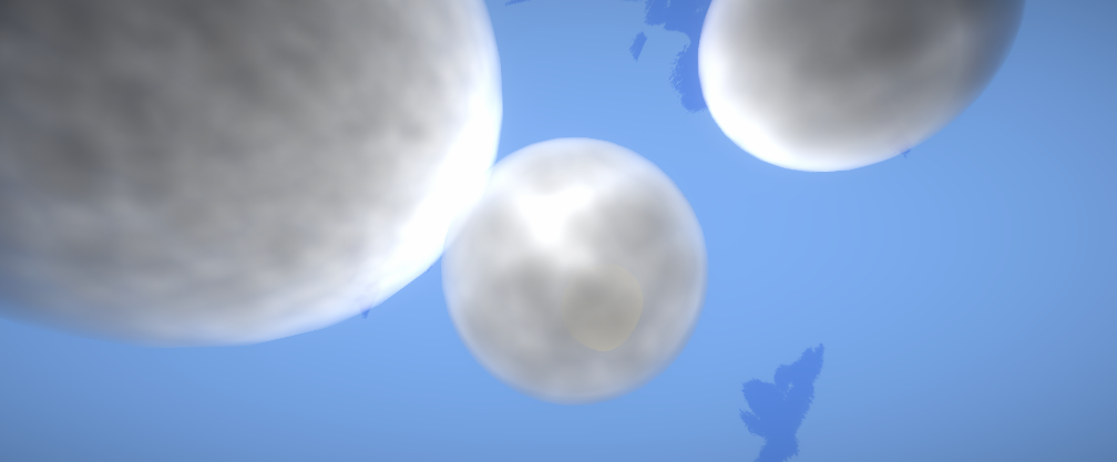
A hard border fits the background more, meaning a cutoff needs to be added for points above a specific transmittance value
```
// added at the bottom of the march function
if (transmittance > cutoff) {
  transmittance = 1;
}
```
Example with threshold at 0.5

§ Final Renderings

At steps = 50

↗
At steps = 25

↗
At steps = 10

↗
At steps = 4

↗
The first three renderings do not look that different, mainly because the texture scale is set to a very small value. For higher resolutions (and more frequency multiples than just two) the rendering might look different.
Without rigorously testing performance, 10 steps is where the framerate drop begins to be noticeable
Most of the performance should be taken up by texture sampling, as per-step computations are relatively light
- By the nature of the ray marching the number of density sampling is O(steps^2)
- This could be helped if different channels in the noise texture were already scaled according to frequency, this way only one sample is needed.

§ Conclusion

§ Answering the Challenges

Viewing angle
- Cloud lighting looks believable at most viewing angles
Occlusion
- Artifacts still exist between adjacent clouds: a certain cloud could leap before an adjacent cloud when it "wins" the Z-test after a small angle variation
- The fainted edges are not entirely convincing
Cost
- Constant-step for loops are unwrapped statically by the compiler, meaning there is little branching
- Step count can be low enough (4 for both stage I and II) without causing visual issues
Variation:
- Noise looks random enough
Stylistic
- Several techniques were used to make the cloud look cartoonish
- It is hard to balance between contrast and liveliness (grays look too dull but are necessary for giving "mass" to the cloud)

§ Future Improvements

Connecting step count with Unity's Quality settings
Using fiber-like textures to further stylize the noise
Fixing occlusion issues for adjacent clouds

::

Technical-art

::